Mortality monitoring in Switzerland
DOI: https://doi.org/10.4414/SMW.2021.w30030
Rolf
Weitkunat, Christoph
Junker, Seraina
Caviezel, Katharina
Fehst
Federal Statistical Office, Neuchâtel, Switzerland
Summary
The Federal Statistical Office publishes weekly national and regional mortality reports online for Switzerland for the age groups 0 to <65 and 65+ years, which refer to deaths up to 9 days prior to the publication date. In addition to observed numbers of death events, expected numbers are reported, which allows detection of periods of excess mortality and its quantification. As with previous periods of excess mortality, in 2020 the monitoring detected and quantified excess mortality during the two waves of the SARS-CoV-2 epidemic in Switzerland. During the year, the epidemic resulted in well over 10% more deaths than expected, mainly in individuals aged 65 years and above. Because of the profound impact of the epidemic, interest in the weekly mortality publication and its underlying methodology increased sharply. From inquiries and from newspaper and tabloid publications on the matter it became abundantly evident that the principles of the mortality monitoring were not well understood in general; mortality monitoring was even regularly confused with cause of death statistics. The present article therefore aims at elucidating the methodology of national mortality monitoring in Switzerland and at putting it into its public health context.
Introduction
Since May 2015, the Swiss Federal Statistical Office (FSO) has published, every Tuesday at 14:00, the weekly numbers of domestic deaths of Swiss residents, separately for age groups 0 to <65 and 65+ years, both graphically and numerically. In April 2020, the FSO has launched an additional experimental publication, where the same information is now also provided for the seven Swiss NUTS-2 (Nomenclature des unités territoriales statistiques) regions Lake Geneva, Espace Mittelland, Northwest Switzerland, Zurich, Eastern Switzerland, Central Switzerland, and Ticino. As of February 2021, NUTS-3 (cantonal) data are being published as well.
From about the middle of 2020 to the middle of 2021 the FSO online publication on the weekly number of deaths in Switzerland by age group had become one of the most frequently referenced sources of information on the SARS-CoV-2 pandemic in Switzerland. As in many other countries, it became clear that excess mortality encompasses all causes of death, therefore quantifying the overall impact of COVID-19 on mortality [1–3]. At the time, a large number of inquiries from the press as well as from the public were addressing all aspects of the methodology. Many questions concerned the differences between the weekly numbers of deaths and the annual cause of death statistics, the underlying data flow and data processing, the calculation of the expected numbers of deaths and of the confidence intervals around these expected numbers, the reasons for the unavailability of cause of death statistics for the current year and the previous year, the reasons for and the extent of reporting delays, the determination of excess mortality, and the relationship between excess mortality on the one hand and of deaths due to SARS-CoV-2 infections on the other. As became evident in the course of the pandemic, mortality and cause of death statistics were quite often confused and neither was commonly well understood. The present contribution therefore summarises the methodology underlying the FSO's reporting on the weekly number of deaths in Switzerland and in addition briefly recapitulates mortality during the pandemic in 2020 to mid-2021.
Collection of mortality data
The collection and reporting of mortality data and cause of death information entails two processes: a first, relatively fast process of registering and reporting each case of death occurring in Switzerland (mortality monitoring), and a second, more time-consuming process of collecting and processing the corresponding causes of death. Because of the complexity of the processes, it is worth clarifying the fundamental differences in contents and timelines of mortality monitoring on the one hand and cause of death statistics on the other. This requires an overview of the underlying administrative procedures and corresponding data flows, which are depicted in figure 1 and summarised in the following.
When a person dies in Switzerland, the competent civil registration office is notified, usually by the attending physician, by the hospital or nursing home management, or by relatives of the deceased. Every business day, the FSO receives notifications on recent cases of death, including date of death, location and age of the deceased. As of 2005, this is by the civil registration offices (coordinated by the Federal Office of Civil Status, FOCS) updating a deceased person's civil registration record in the national Infostar database. This first part of the collection of mortality data is thus centred on registering and processing events and the corresponding personal data. It is the basis of the weekly updates through the FSO's mortality monitoring. The focus of the present paper is on this fast part of the mortality data collection and reporting. However, before the details of this process are addressed, a brief overview will be given of the second, more time-consuming part, which leads to the cause of death statistics.
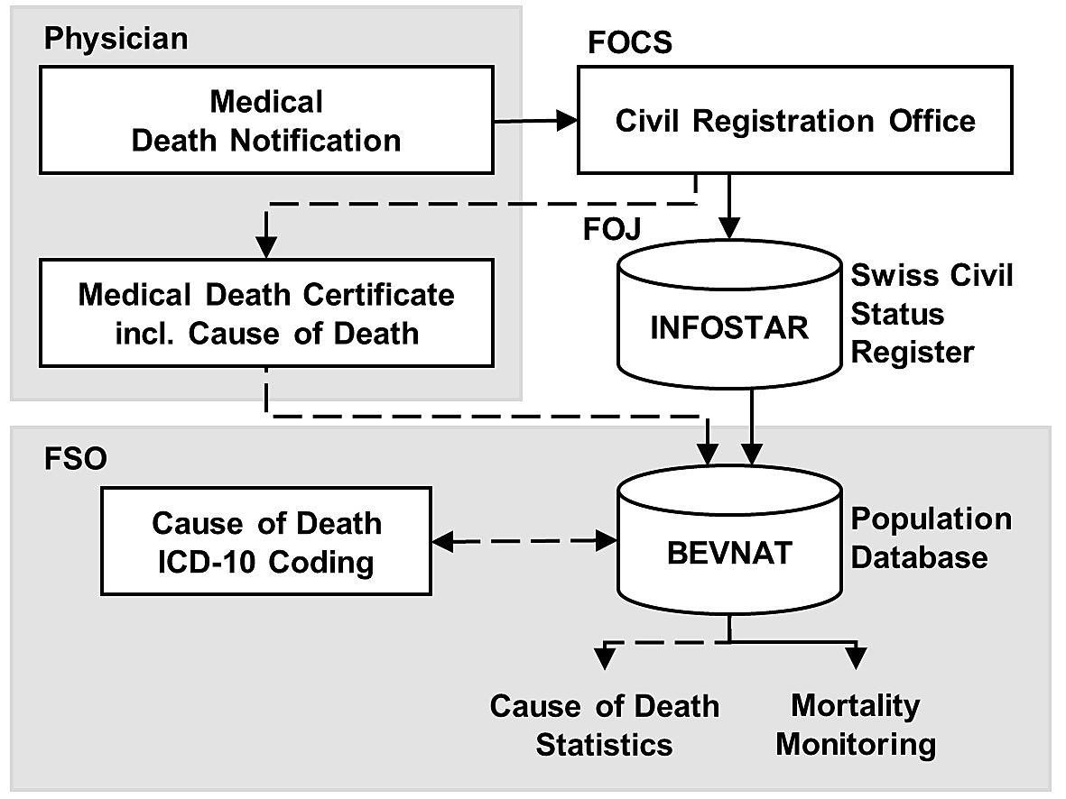
Figure 1 Administrative and informational paths leading from a death notification to the generation of weekly mortality updates and eventually to cause of death statistics. The Federal Office of Statistics' (FSO) BEVNAT database receives nightly updates through the Federal Office of Justice (FOJ) INFOSTAR register, allowing for timely mortality monitoring with weekly reports. Cause of death statistics require additional processing and coding, implying a longer publication delay.
In parallel to the rapid update of the civil status register database Infostar for a given case of death, the civil registration office issues a request and form containing the identification number of the deceased to the attending physician for providing a medical death certificate. The death certificate is to be sent directly to the FSO, either on paper or electronically (currently about 39% of the death certificates). The medical death certificate comprises different relevant causes of death: the underlying disease or root cause, the immediate cause of death or secondary disease and, if applicable, concomitant diseases. These diseases are noted in longhand on the medical certificate, and the FSO then codes them according to the rules of the International Classification of Diseases (ICD-10) of the World Health Organization (WHO). The ICD-coded cases are the basis of the FSO's annual statistical publication on causes of death. In the last few years, the annual number of deaths in Switzerland was just below 68,000, the threshold of 70,000 exceeded for the first time only in 2020. As ICD coding is a complicated and time-consuming process, requiring specialised personnel and involving collecting of outstanding death certificates and issuing of queries for unclear or missing information, the elaboration of the cause of death statistics requires a thorough processing of each individual death certificate. As presumably has become clear at this point, mortality monitoring (merely considering the event itself rather than the cause of death) is a much timelier affair, and updated statistics can be published weekly, taking into account deaths from 9 or more days ago.
Mortality in 2020 and 2021
Owing to the FSO operation of national-scale mortality monitoring and of online publishing of the results on a weekly basis, the type of information contained in figure 2 was available throughout the epidemic, weekly updates lagging behind the current development by less than 2 weeks. As previously during influenza epidemics and heatwaves, the mortality monitoring system has demonstrated its importance as a reliable and timely source of fundamental public health information. The FSO also shares the weekly numbers of deaths in Switzerland with the European Mortality Monitoring Project (EuroMOMO) [4]. This collaborative network started its operations in 2008 and today provides weekly mortality statistics on 27 European countries, leveraging the regional and national mortality monitoring to the international level.
During the SARS-CoV-2 pandemic, the Swiss Federal Office of Public Health (FOPH) started to publish daily incidence and mortality counts, the latter referring to individuals who died after a positive test for the virus. The parallel publications gave rise to questions as to how the two mortality statistics would relate to each other, observers frequently failing to grasp the fundamental difference. Whereas mortality monitoring is based on the continuous complete inventory of deaths collected through the civil registration system, irrespective of the cause of death, the FOPH's daily reports on deaths related to COVID-19 are based on mandatory reports of test-positive cases provided by physicians, hospitals, healthcare institutions and laboratories in Switzerland according to WHO rules.
During the first wave of the SARS-CoV-2 pandemic in Switzerland, from 16 March 2020 (week 12) to 19 April 2020 (week 16), mortality monitoring has received intensive attention by the press and by the public. During these 5 weeks, the numbers of people having died at age 0 to <65 years and at 65 years and above (65+) were more than 12% and 26%, respectively, higher than expected. The week with the highest excess mortality during the first wave was week 14 (30 March to 5 April 2020), when the excess was 46% in people 65+ years of age. During the second wave, taking off in week 43 and lasting until week 4 of 2021, 47% more deaths than expected occurred in this age group, the week with the highest weekly excess mortality being that of 16 to 22 November 2020 (week 47), when 70% more people than expected died in the 65+ years age group. During both waves, the time-course of the epidemic differed considerably across regions, with the onset of the first wave in 2020 ranging from week 11 (Lake Geneva region and Ticino) to week 16 (Central Switzerland), and that of the second wave ranging from week 43 (Espace Mittelland) to week 45 (Northwestern Switzerland). Likewise, the durations of the two waves were quite different among the regions, the first and second wave lasting 1 week and 14 weeks, respectively, in Central Switzerland, and both waves lasting 9 weeks in the Lake Geneva region.

Figure 2 Federal Statistical Office web publication on the weekly number of deaths in Switzerland by age group (with completed years of life), from week 1, 2020 to week 29, 2021. The connected dots represent numbers of observed deaths per week; the bands are two-sided 99% confidence intervals around the predicted numbers for the corresponding weeks (data status 03 August 2021) [5].
Observed and expected numbers of deaths
As there is some lag in the registration of cases of death with the local civil registration offices, the most recent numbers covered in the weekly publications refer to the week ending 9 days prior to each new publication. Also, and for the same reason, the numbers for the most recent reporting week and for the 4 weeks preceding it are projections, based on the numbers registered thus far as well as on the distribution of the registration delays over the previous one and a half years. Along with these observed numbers (albeit, as pointed out, the most recent ones being projections), the expected numbers of deaths per week are published.
Mortality monitoring hence not only involves registering and backward-projecting observed numbers of deaths, but also forward-predicting future expected numbers of deaths, the difference between projection and prediction being relevant for understanding the methodology. Projecting what the incompletely registered final numbers of deaths for recent weeks will eventually be once the registration is completed amounts to estimating what the past will look like in the future. In contrast, predicting what the numbers of deaths in future weeks will eventually be is proper forecasting, amounting to estimating what the future will most likely look like.
It might appear that the publication of the weekly numbers of observed and expected deaths in Switzerland as a whole and in the regions should be a straightforward enough affair. However, the actual generation of the underlying statistics involves a few technical aspects, which seem to warrant a somewhat more detailed description as provided in the following, and schematically illustrated in figure 3. The technical details of the implementation and parameterisation of the procedure are described in appendix 1. Estimating the expected number of deaths in each week of the present year is not based on a closed formula, but on a complex algorithm. The procedure is performed for each NUTS-2 region to determine the expected number of deaths per calendar week of the ongoing (prediction) year. Subsequently, the values of the regions are summed up for the whole of Switzerland.
Overall, the procedure consists of two consecutive passes, the first pass estimating the overall mortality level of the present year for which predictions are generated, the second pass estimating calendar-weekly numbers of deaths. Splitting the estimation into two passes allows secular mortality trends (including demographic changes, population growth and increasing life expectancy) to be accounted for in the first pass and seasonality in the second.
Before the final expected numbers of deaths in each week of the current (i.e., the to be predicted) year are obtained, separately for age groups 0 to <65 and 65+ years as well as for all of Switzerland and for different regions, predicted numbers are thus in fact estimated twice over.
In the first pass, estimates are from a regression model to predict the total number of deaths in the current year from the annual numbers of deaths over the past 5 years, after reducing random year-to-year variation by smoothing over these annual numbers. A period of data consisting of the 5 previous years is considered, which strikes an experiential balance between reflecting ongoing trends with sufficient precision, while still being sensitive to short-term changes when they occur. This first pass of the estimation process is conducted separately for the 7 NUTS-2 regions and for 11 age groups, to account for regional differences and for secular trends, which may impact certain regions and age groups more than others. Because of this stratification, the estimates reflect changes in mortality over time caused in part by changes in the size and age distribution of the population.
The second pass estimates are weekly median numbers of deaths obtained over the past 10 years, separately for age groups 0 to <65 and 65+ years, and smoothed over the course of the current year. Ten years of data are required to provide stable weekly estimates in the second pass. Day-to-day estimates for the current year are obtained subsequently from these smooth weekly medians, taking into account the mapping of the weekdays onto the calendar dates of the days of the current year. The daily estimates are finally weighted, based on the first-pass annual estimates, such that their sum corresponds with the first-pass expectation for the current year. The so calibrated daily estimates are finally aggregated by calendar weeks, and regional estimates are further aggregated to yield national-level estimates. Finally, confidence intervals are calculated for the weekly age group-specific expected numbers, both at the national and the regional level.
In more detail, the procedure to estimate expected numbers of deaths for each week of the current (i.e., the to-be-predicted) year consists of the following 13 steps:
Step 1: Deaths in the past years are counted, separately for each of the 11 age groups (0 to <5 years; 5 to <15; 15 to <30; 30 to <65; 65 to <70; 70 to <75; 75 to <80; 80 to <85; 85 to <90; 90 to <95; 95+).
Step 2: The numbers of deaths per age group (fig. 3a) are smoothed across calendar years (fig. 3b) through locally weighted regression [6].
Step 3: The number of deaths per age group for the prediction year is estimated by Poisson regression based on the past 5 years (fig. 3c).
Step 4: Separately for the 0 to <65 and 65+ year age groups, the predicted numbers of deaths for the prediction year (first-pass estimates) are aggregated across the initial 11 age groups.
The subsequent steps are conducted separately for the two resulting age groups 0 to <65 and 65+ years:
Step 5: Deaths per calendar week are counted for the past 10 years.
Step 6: Median numbers of deaths are calculated for each calendar week (fig. 3d).
Step 7: The median numbers of deaths per calendar week are smoothed over the year through locally weighted regression (fig. 3e).
Step 8: Each calendar week's smoothed medians are divided by 7 to obtain per-day expected numbers of deaths.
Step 9: Per-day expected numbers of deaths are allocated to the calendar weeks of the prediction year.
Step 10: The number of deaths expected for the prediction year (second-pass estimates) is obtained by aggregating the per-day expected numbers of deaths.
Step 11: The first-pass predicted deaths (step 4) are divided by those estimated in the second pass (step 10).
Step 12: The expected deaths allocated to the calendar weeks of the prediction year in step 9 are multiplied by the factor determined in step 11 (fig. 3e).
Step 13: For each calendar week, a 99% Poisson confidence interval is determined for the final number of expected deaths as calculated in step 12 (fig. 3f).
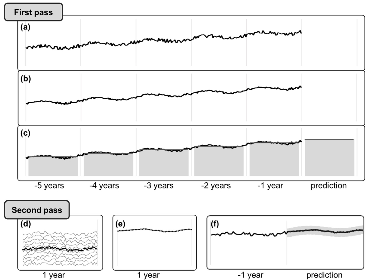
Figure 3 Schematic of the calculation of the expected number of deaths for a given age group in each week of the present year of mortality monitoring. In the first pass, observed numbers of deaths (a) are smoothed across the previous 5 calendar years (b) and the expected number for the current (prediction) year is estimated (c; years indicated by vertical bars). In the second pass, the weekly median numbers of deaths (dotted line) are calculated (d), then smoothed and calibrated to correspond to the expected level estimated in the first pass (e). Finally, a confidence band is determined for the weekly numbers of expected deaths of the current (prediction) year (f).
It should be noted that the expected mortality counts for the weeks of the current calendar year (the prediction period) and, by implication, of the number of excess deaths is contingent on the estimation methods being used. A considerable number of statistical approaches have been used by various institutions, including time-series analysis, fitting sine and cosine functions to account for the seasonal variation, and parametric as well as robust regression methods explicitly accounting for population growth and demographic changes. Additional data processing methods have been deployed in various combinations, such as smoothing adjacent data points through spline functions or locally weighted regression and models for short-term projections of observed numbers of deaths for recent periods with registration delays. Methods also differ with respect to how confidence intervals are calculated, including the use of traditional frequentist, Bayesian, or resampling methods. Other differences across models include the number of past years used to predict the mortality of the current year, the definition of the event date (death vs registration of death), and the degree of precision for calculating confidence intervals. Often, some implementation of an overdispersed Poisson generalised linear model with spline terms is used, which was initially proposed by Farrington et al. [7] and improved by Noufaily et al. [8], for example by the US Centers for Disease Control and Prevention (CDC) [9]. EuroMOMO [10], reanalysing the data of all member states for comparability, uses a Poisson time-series regression with the number of weekly deaths regressed on a linear trend term over 3 to 5 years and, for age groups of 15 years and above, on a sine function term reflecting annual cyclical seasonality. Prediction intervals are calculated based on the standard deviation of the model residuals.
The considerable number of methodological options and the various ways in which mortality monitoring is being conducted currently gives rise to the question as to how good the Swiss mortality monitoring is by international standards. Unfortunately, quality indicators of the mortality monitoring systems as implemented in different countries are, to put it mildly, hard to come by. Although this makes a head-to-head comparison difficult, it is still possible to assess the quality of the Swiss mortality monitoring in absolute terms. Table 1 contains the annual numbers of observed and model-based expected deaths, separately for the two age groups 0 to <65 and 65+ years of age.
Table 1Performance characteristics of the Swiss national mortality monitoring based on the proximity of the annually expected and the observed numbers of deaths in the period of 2010 to 2019.
|
Age group:
|
0 to <65 years
|
65+ years
|
|
Year
|
Observed
|
Expected
|
Difference
|
% difference
|
Observed
|
Expected
|
Difference
|
% difference
|
| 2010 |
9679 |
9623 |
56 |
0.6 |
52,359 |
51,719 |
640 |
1.2 |
| 2011 |
9343 |
9501 |
–158 |
–1.7 |
52,077 |
52,591 |
–514 |
–1.0 |
| 2012 |
9432 |
9242 |
190 |
2.1 |
53,916 |
52,670 |
1246 |
2.4 |
| 2013 |
9336 |
9144 |
192 |
2.1 |
54,881 |
54,109 |
772 |
1.4 |
| 2014 |
8910 |
9047 |
–137 |
–1.5 |
54,135 |
55,526 |
–1391 |
–2.5 |
| 2015 |
9339 |
8981 |
358 |
4.0 |
58,726 |
56,621 |
2105 |
3.7 |
| 2016 |
8796 |
8785 |
11 |
0.1 |
55,293 |
57,298 |
–2005 |
–3.5 |
| 2017 |
8768 |
8648 |
120 |
1.4 |
57,119 |
57,073 |
46 |
0.1 |
| 2018 |
8798 |
8562 |
236 |
2.8 |
57,271 |
57,583 |
–312 |
–0.5 |
| 2019 |
8472 |
8530 |
–58 |
–0.7 |
58,338 |
57,741 |
597 |
1.0 |
The assessment of the results shown in table 1 has to take into account that the absolute and relative differences between observed and predicted numbers do not reflect the net model performance, but are obviously also affected by periods of excess or deficit mortality, in either or both age groups. For example, in 2015 there was a substantial influenza epidemic in Switzerland, having led to more deaths than expected for the year. Consequently, the difference between observed and expected numbers of deaths was the highest over the 10-year period, the magnitude not pointing at a poor fit of the mortality prediction but rather at its high sensitivity to periods of excess mortality. Aggregated across the whole 10-year period, the deviance is 0.9% and 0.2% in the age groups 0 to <65 and 65+ years, respectively, the grand total deviance being 0.3%. Based on this, it appears to be rather difficult to disagree on the flat out excellent performance of the Swiss mortality monitoring statistical prediction methodology.
Discussion
The FSO's operation of monitoring the mortality on a weekly basis is a fundamental and highly informative cornerstone of public health surveillance in Switzerland. It provides continuous information on the time course of mortality at different levels of temporal, spatial, and demographic resolution: over years, months, and seasons, within years, in recent weeks, in the total population, in different age groups, nationwide, as well as regionally. It provides guidelines for evaluating deviations of the weekly number of deaths from the statistically expected number in terms of whether the magnitude of the deviation is more likely random or rather due to a substantial population-wide change in mortality. Furthermore, mortality monitoring supports identification of demographic and geographic focal points, thus facilitating the planning of public health countermeasures and the identification of possible causes for excessive mortality if it occurs.
From a methodological point of view, mortality monitoring rests on two epistemologically different pillars. Firstly, it is based on actual numbers of deaths. More than 85% of deaths are usually registered after 9 days, 97.5% after 40 days, and the remaining 2.5% of reports usually arrive within a year, mostly within the year of death. Even with the actual numbers of deaths in the most recent 5 weeks partially based on projections, the actual (observed) numbers of deaths per week thus essentially represent measurements, i.e., empirical facts, for all practical intents and purposes.
Secondly, mortality monitoring also rests on predicted numbers of deaths. Predictions are built on actual historical mortality, but they certainly also rest on statistical modelling. Due to that modelling part, predicted numbers are method-dependent expectations, i.e., quantitative hypotheses, rather than empirical facts. The actual predictions made by a statistical model reflect two fundamental methodological decisions, one being the choice of the prediction model and its parametrisation, the other the credibility requested for the predictions. Although certainly considering the state of the art, arbitrariness still lies in the choice of the type of the statistical model (e.g., regression, resampling, stochastic simulation, etc.) and in the methodological details actually deployed for making the model-based estimations. These details include (but are not restricted to) the subset, stratification (for example, by age groups), and the temporal resolution of the historical data used; the specifications of the deployed data model (e.g., linear, polynomial); the degree of smoothing imposed on the historical data points; the loss function and the optimisation method selected for estimating the model parameters; the choice of methods for consolidating sub-models.
The other fundamental decision regards the degree of credibility one requires the model-based predicted numbers of weekly deaths to have. As the process of dying is, at least at the real-world scale of scrutiny, far from being deterministic (for example, by not exclusively depending on age) but entails a substantial stochastic component, the number of deaths occurring in a given week comprises an irreducible random component. Thus, and due to the shortcomings of the selected model and the details of its specification, even a model-based hindcasting of historical deaths inevitably results in some degree of deviation of the expected from the observed weekly numbers of death. Based on this deviation, it is possible to determine the degree of precision of the model-based point estimates. This precision (the standard error) can in turn be used to calculate a confidence interval around the weekly numbers of deaths estimated with the model, as pointed out above. The more certain one desires to be with regard to the point estimate being within the limits of the confidence interval, the wider the interval necessarily becomes. As absolute certainty entails infinite width, fixing the desired level of certainty implies a trade-off and thus an unavoidable choice, and one unfortunately beyond the realm of statistical methods at that. The choice of the desired degree of certainty regarding the confidence interval of the predictions is important, as the excess mortality determined from the observed and the predicted numbers depends on its width.
Would one naively trust the model predictions, this would have two crucial implications. Firstly, there would be zero percent certainty that the point prediction is correct; secondly, any number of observed deaths beyond the predicted level would have to be considered to represent excess mortality. This would of course entirely neglect the described random variation that comes with the phenomenon at hand, and thus the inevitable lack of precision of the prediction. The Swiss mortality monitoring uses a 99% and thus rather conservative (i.e., fairly wide) confidence interval to minimise the false alarm rate, not least because the overall false alarm rate depends on the total number of assessments conducted each week in different age and regional subsets. Only when in a given comparison the observed number of deaths exceeds the upper limit of the 99% confidence interval of the corresponding predicted number, is excess mortality detected. Of note, although the decision as to whether or not excess mortality is declared depends on the width of the confidence interval around the predicted number, the magnitude of the excess mortality (once it is declared) itself does not. The reason is that, if excess mortality is detected, it is always quantified by the difference between the observed and the expected number of deaths, irrespective of the upper limit of the confidence interval.
Given that it considers all cases of death, the mortality monitoring is comprehensive. At the same time, its sensitivity to dynamic mortality variations is limited by its temporal resolution, which results from downsampling the daily flow of registered events to weekly numbers. Consequently, mortality monitoring is per se not a panacea for detecting all kinds of changes in population mortality, its dynamic range being clearly optimised for detecting medium fast changes. Based on the sampling rate of 52 discrete data points per year, mortality monitoring sensitively detects mortality changes manifesting over a biweekly or somewhat less than biweekly period (the Nyquist-Shannon theorem). At the low frequency end of its dynamic range, mortality monitoring is also capable of detecting trends manifesting in less than a year. The passband for detectable changes in mortality results from both the mortality trend over the recent 5 years as well as the annual seasonality being considered in the prediction method. By combining both trajectories, the confidence band of expected deaths smoothly traces the actual mortality through the weeks of a year. However, the ability of the procedure to detect trends deteriorates as soon as mortality deviates only slightly from the predictions from week to week. Smaller changes that only accumulate over several weeks may well go undetected if the trend is not so strong that its weekly manifestations exceed the upper confidence interval limits of the predictions.
A limitation of mortality monitoring, inherent in the reporting delays, is its limited timeliness. Based on reporting delays observed during the previous one and a half years, current delayed reporting is compensated for by adjusting the figures for the 5 most recent reporting weeks. However, to avoid excessive uncertainty, such projections are not undertaken for the week directly preceding the current calendar week. Consequently, the last reported week always ends 9 days before the update on Tuesday of the current calendar week. Population-level exposures that affect mortality are therefore not detected by mortality monitoring earlier than 1 to 2 weeks after the event. Depending on the nature of the event, this may be too slow for timely public health interventions. In the SARS-CoV-2 pandemic, mortality-based monitoring lagged 3 to 6 weeks behind the actual infections.
Although mortality monitoring is an important, valuable and reliable statistical routine operation, the methodological development is by no means concluded. In 2020, we started increasing the regional resolution of the process, first by now also monitoring NUTS-2 regions and subsequently by extending the scope to NUTS-3 regions (i.e., cantons). In the future, the monitoring might be able to cover the level of districts and possibly communities, even though it remains to be seen how reliably mortality can be predicted as the size of the regional aggregates decreases and the signal-to-noise ratio consequently increases.
The year 2020 was remarkable also with regard to the established prediction methodology. Periods of increased mortality have in the past never appeared to substantially impact the mortality predictions of subsequent years, but this has recently changed. During the SARS-CoV-2 pandemic, Switzerland has suffered a toll well in excess of 10% more deaths than expected. When running the described algorithm to predict the expected numbers of deaths per week for 2021, we were surprised to note that the previous year's tremendous excess mortality had indeed led to an implausible upward jump of the predicted mortality trajectory throughout 2021. To sustain the mortality monitoring process amidst the second wave of the pandemic, we had no better option than to reuse the 2020 prediction for 2021 also. Naturally, we are now further developing the mortality prediction method so that it can absorb shocks of the magnitude experienced in 2020 without producing implausible forecasts for subsequent years. A practical approach appears to be replacing the observed numbers of deaths by the predicted ones for periods of excess mortality. As in the past, it is the precision of the forecasts over time by which the revised method will then have to be assessed.
The FSO's mortality monitoring has become one of the most widely quoted statistics during the pandemic, with a focus of public interest on excess mortality. Not all of the interpretations were entirely adequate, which is unsurprising, given the underlying conceptual and methodological complexities. For example, it is easy to overlook the fact that the level of mortality (and hence excess mortality) observed at a given time depends on previous levels. People whose death has been advanced, for example by an infection during a pandemic, are simply unavailable to contribute to the death count in any subsequent period, the phenomenon being referred to as “mortality displacement” or "harvesting effect" [11]. Also, while mortality monitoring quantifies excess deaths in certain regions and time periods due to these deaths occurring earlier than expected, it does not quantify the amount of lifetime lost.
In spite of this, the biggest advantage of mortality over other population health indicators is its completeness and apparent simplicity; all deceased cases make up the final mortality count. However, this straightforwardness is indeed deceiving. Mortality in general and excess mortality during a pandemic in particular are conglomerates of many factors. Excess mortality comprises not merely the immediate and direct effects of the virus, but also its delayed and indirect effects, the latter including the dynamic spread of the virus, both influenced by as well as in turn influencing transmission-relevant behaviour. Other factors include environmental effects (e.g., season, temperature), the age and health of the population, as well as the intended and unintended effects of counter-measures at the individual (e.g., immunisation, masks, distancing) and population level (e.g., contact restrictions, lockdowns), including the adherence patterns in the population. Quantifying the effects of counter-measures on mortality is complicated by the fact that these measures are pleiotropic by having more effects than merely reducing the transmission of the targeted virus. Although these effects may in principle include unintended ones, most of the unspecific effects might very likely contribute to reducing mortality more broadly, for example by possibly reducing the number of accidents (traffic and otherwise) and by lowering the transmission of infectious diseases in general (including the seasonal influenza).
For these reasons, quantifying the virus-specific epidemic death toll is not viable solely based on excess mortality. Likewise, the mortality prevented by specific public health counter-measures cannot be derived through mortality monitoring alone. To achieve the former, in addition to the numbers also the causes of deaths are required. The latter question can only be tackled by comprehensive comparative analyses of various types of data collected during the pandemic, with the data obtained through mortality monitoring certainly playing an important role.
Rolf Weikunat, PhD
Federal Statistical Office
Espace de l'Europe 10
CH-2010 Neuchâtel
rolf.weitkunat[at]bfs.admin.ch
References
1.
Beaney T
,
Clarke JM
,
Jain V
,
Golestaneh AK
,
Lyons G
,
Salman D
, et al.
Excess mortality: the gold standard in measuring the impact of COVID-19 worldwide? J R Soc Med. 2020 Sep;113(9):329–34. https://doi.org/10.1177/0141076820956802
2.
Nørgaard SK
,
Vestergaard LS
,
Nielsen J
,
Richter L
,
Schmid D
,
Bustos N
, et al.
Real-time monitoring shows substantial excess all-cause mortality during second wave of COVID-19 in Europe, October to December 2020. Euro Surveill. 2021 Jan;26(2):2002023. https://doi.org/10.2807/1560-7917.ES.2021.26.1.2002023
3.
Islam N
,
Shkolnikov VM
,
Acosta RJ
,
Klimkin I
,
Kawachi I
,
Irizarry RA
, et al.
Excess deaths associated with covid-19 pandemic in 2020: age and sex disaggregated time series analysis in 29 high income countries. BMJ. 2021 May;373(1137):n1137. https://doi.org/10.1136/bmj.n1137
4.
EuroMOMO
. 2021. doi: https://www.euromomo.eu/
5.
FSO
. 2021. Mortality, causes of death. doi: https://www.bfs.admin.ch/bfs/en/home/statistics/health/state-health/mortality-causes-death.html
6.
Cleveland WS
. Robust locally weighted regression and smoothing scatterplots. J Am Stat Assoc. 1979;75(368):829–36. https://doi.org/10.1080/01621459.1979.10481038
7.
Farrington CP
,
Andrews NJ
,
Beale AD
,
Catchpole MA
. A statistical algorithm for the early detection of outbreaks of infectious disease. J R Stat Soc Ser A Stat Soc. 1996;159(3):547–63. https://doi.org/10.2307/2983331
8.
Noufaily A
,
Enki DG
,
Farrington P
,
Garthwaite P
,
Andrews N
,
Charlett A
. An improved algorithm for outbreak detection in multiple surveillance systems. Stat Med. 2013 Mar;32(7):1206–22. https://doi.org/10.1002/sim.5595
9.
CDC
. Excess deaths associated with COVID-19. Atlanta, GA: US Department of Health and Human Services, CDC, National Center for Health Statistics. 2020; doi: https://www.cdc.gov/nchs/nvss/vsrr/covid19/excess_deaths.htm
10.
Gergonne B
,
Mazick A
,
O’Donnell J
,
Oza A
,
Cox B
, et al.
A European algorithm for a common monitoring of mortality across Europe. Work package 7 report. Copenhagen: Statens Serum Institut. 2011.
11.
Huynen MM
,
Martens P
,
Schram D
,
Weijenberg MP
,
Kunst AE
. The impact of heat waves and cold spells on mortality rates in the Dutch population. Environ Health Perspect. 2001 May;109(5):463–70. https://doi.org/10.1289/ehp.01109463
12.
Farr W
. Progress of epidemics – epidemic of smallpox. Boston Med Surg J. 1841;24(4):54–7. https://doi.org/10.1056/NEJM184103030240402
Appendices
Appendix 1: Technical and statistical details
Appendix 2: Historical background
The appendices are available in the PDF version of this article.