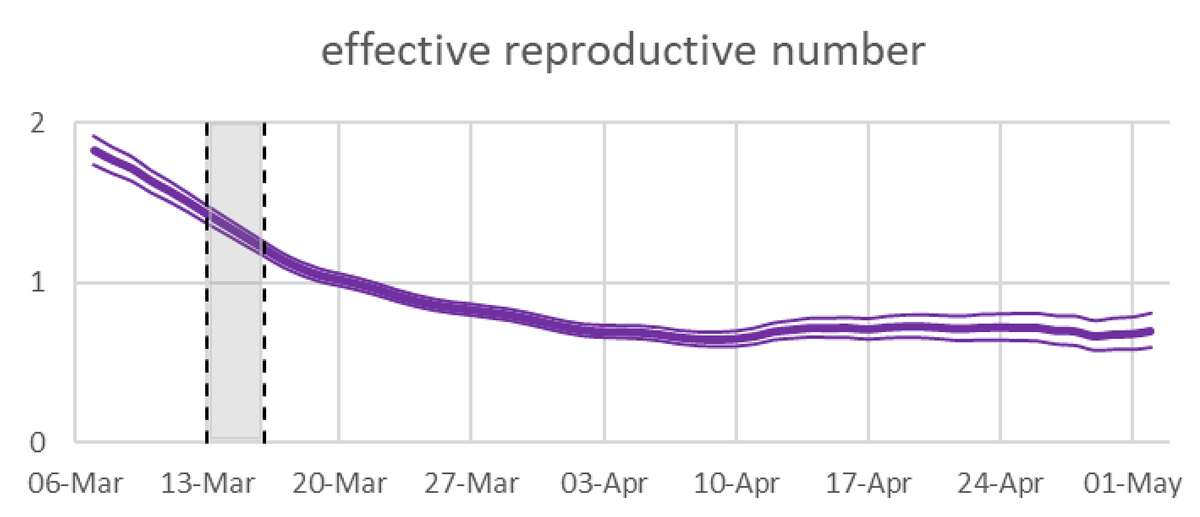
Figure 1 Effective reproductive numbers in Switzerland as shown in the real time monitoring on 13 May 2020. Mean and 95% uncertainty intervals are estimated on confirmed cases [1]. The shaded region is the onset of strong public health measures.
DOI: https://doi.org/10.4414/smw.2020.20307
The effective reproductive number Rt of COVID-19 is determined indirectly from data that are only incompletely known (fig. 1). Approaches based on reconstructing these data by sampling time lags from suitable distributions introduce noise effects that can result in distorted estimates of Rt . This, in turn, may lead to misleading interpretations of the efficacy of the various measures taken to limit COVID-19 transmission. We discuss in some detail a study used for real time monitoring of the reproductive number in Switzerland [2].
Figure 1 Effective reproductive numbers in Switzerland as shown in the real time monitoring on 13 May 2020. Mean and 95% uncertainty intervals are estimated on confirmed cases [1]. The shaded region is the onset of strong public health measures.
We argue that the method used to derive the above curve is systematically flawed and leads to an underestimation of the efficacy of the lockdown. The method adopted by the Robert Koch Institute suffers from similar deficiencies, their impact is however smaller.
The daily varying effective reproductive number Rt is often used to monitor the spread of epidemic diseases such as COVID-19. It measures the expected number of secondary infections on day t due to a single infected individual and is given by
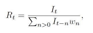
where It is the number of new infections on day t (and equally It − n the number of infections on day t − n and so on), and the wn are the infection intensities, i.e. wn is the probability that a secondary infection was contracted from a person who got infected n days earlier. Whereas the infection intensities can be fitted to available data, the It are not observable directly, unless representative proportions of the population were tested on a daily basis. Therefore, they need to be inferred indirectly from some other data.
There are different schemes to reconstruct the It from the data, such as the classical statistical inference methods. In the present article we concentrate on schemes that are based on the idea of a “mechanical” reconstruction of the infection data by sampling time lags of observed data from suitable distributions. In the context of the current COVID-19 pandemic, such schemes have been implemented in different ways by various groups in different countries.
In the following section, we present these schemes and show how they systematically introduce noise into the true data. In the remaining sections we examine the impact of the noise on the reproductive numbers calculated from these data.
We exemplify the scheme and how it introduces noise into the data by the version implemented by Scire et al. [3], which is very similar to the implementation by Abbott et al [4]. For the sake of clarity, we limit our exposition of the scheme to the observables C t , the number of confirmed cases on day t. The other observables used analogously by the group are hospitalisations and deaths. Moreover, as our focus is on the days around 17 March, when the lockdown started, and as more than 2 months have passed since then, we restrict our exposition to those days of infection where all infections can be assumed to be confirmed by the actual date of the monitoring. According to the parameters used by the group, 95% of the cases are confirmed within 20 days after infection. For their method of extending the reconstruction to later days we refer again to their article.
Now, let X denote the incubation time of a randomly drawn case, i.e. the time between infection and symptom onset, and analogously Y the time between symptom onset and confirmation. The distributions of X and Y result from fitting to available data; see [2] and references therein. Then for every confirmed case α one samples independently a xʹa from the distribution of X and a yʹa from the distribution of Y.
The reconstructed infection day iʹa of this case a is then simply the day when the virus infection was confirmed minus (xʹa + yʹa ). Counting the number of cases that fall now on day t gives the reconstructed It, that we denote by Iʹt . The reproductive numbers calculated from these Iʹ t are denoted by Rʹ t .
That this scheme introduces noise into the true data is seen as follows. We denote the true infection day by i α , the true incubation period by x a and the true time between symptom onset and confirmation by y a . Then we have iʹ a = ia + xa + ya ‒ xʹ a ‒ yʹ a . As the sampled xʹ a and yʹ a are independent of the true xa and ya (because we don’t know these; we just know that they are approximately distributed like X and Y, respectively), the reconstructed iʹ a equals the true “signal” ia plus some ”noise” dʹ a = xa + ya ‒ xʹ a ‒ yʹ a .
As we will see in the following examples, this results in a smoothing of the infection number statistics, which in turn, under certain circumstances, has a significant impact on the reproductive numbers calculated from it. (From a mathematical point of view, this is clear: If all the It are large, then we have C ≅ I ∗ p, where pn = P (X + Y = n), and Iʹ ≅ C ∗p̃, where p̃n = p − n, i.e. Iʹ ≅ I ∗ p ∗ p̃.)
The following example illustrates the effect of this scheme on the reconstructed reproductive number. Assume that I 1 = 128 and R t = 2 for t ≤ 6 and R t = 0.8 for t ≥ 7, and that infectiousness is limited to the day after infection, i.e. w 1 = 1. This yields the “true” infection numbers and reproductive numbers which are illustrated by the red curves in figure 2. For the reconstructed data we take X and Y both to be Gaussian with mean 5 and standard deviation 1. Thus, the “noise” is also Gaussian with mean 0 and standard deviation 2. With this “noise”, the scheme results in the average in the corresponding blue curves.
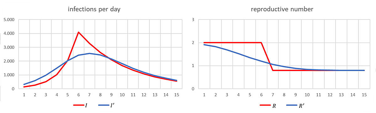
Figure 2 “True” (red) and reconstructed (blue) infection and reproductive numbers.
Of course, the blue curve Rʹ is prone to lead to wrong decisions: If a lockdown caused the sharp decline in R from day 6 to day 7, then the blue curve may suggest that its impact was much less important and that most of the reduction was already achieved before the lockdown. It might even lead to the conclusion that the lockdown was not needed at all and that softer measures in already force before day 6 have had a sufficient effect, whereas in reality they had no effect at all. This in turn could lead to the conclusion that the pandemic can be kept under control by adhering to soft measures only.
We now turn to the situation in Switzerland around 17 March 2020. A calculation based on distributions for the time lags X and Y and the infection intensity as described in [3] yields the following result (fig. 3).
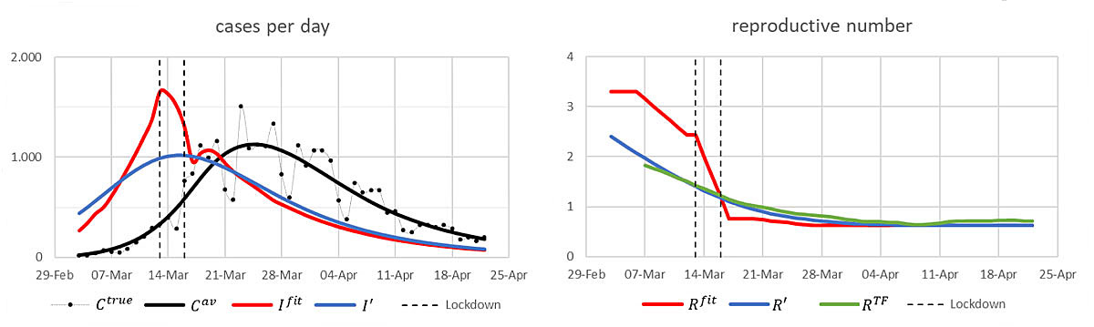
Figure 3 Cases and reproductive numbers in Switzerland around 17 March. See text below for the definition of the curves.
Unlike in the illustrative example above, we cannot start from “true” numbers of new infections. We instead choose the numbers of new infections, denoted by I fit (red curve), in such a way that the resulting expected numbers of confirmed cases C av (solid black curve) fit well the black dots C true which show the actually reported data of confirmed cases [5]. Here, to get C av from the numbers of new infections, we shift forward the infection day of each such case by sampling independently from X and Y. (See appendix 1 for the algorithm used to infer I fit .)
Given I fit , we proceed as in the illustrative example, but, of course, with “noise” according to these X and Y instead of the Gaussian’s used there. This gives the reconstructed numbers of new infections Iʹ (blue curve). Using the infection intensities wn from [3], we calculate the corresponding reproductive numbers R fit and Rʹ. The latter matches well the green curve R TF that shows the estimated mean reproductive numbers, as published on the website [1] on 13 May.
The remarks made above on the illustrative example apply also here. We note also that our red curve of reproductive numbers is in quite good agreement with the results of the inference analysis reported in [6, 7].
Contrary to Switzerland, where, as far as we know, the date of symptom onset of the single cases is not collected systematically, this information is available for the majority of the cases in Germany. For the sake of clarity, we assume here that it is known for all cases. (We refer to [8] for the method applied to the cases with no known date of symptom onset.) Then, the Robert Koch Institute applies the following simpler scheme [8]: The reconstructed infection day ia ̋ of a case a is the day of its symptom onset minus m, where m is the average incubation time. Counting the number of cases that fall now on day t gives the reconstructed I t that we denote by It̋ . The reproductive numbers calculated from these It̋ are denoted by Rt̋ . (As our focus is again on the days around 17 March, we restrict our exposition to those days of infection where all infections can be assumed to be confirmed by the actual date of the monitoring. For a method to extend the reconstruction to later days we refer to [8].)
Of course we can view the subtracted value m as sample from the distribution of the constant time lag X = m. Therefore, this scheme is at least formally very similar to the one adopted by [3].
From the above discussion it is now clear that the so reconstructed infection times ia ̋ = ia + da with ”noise” da ̋ = x a − m lead also to a smoothing of the infection number statistics and thus to misleading reproductive numbers. But it is also intuitively clear, that the impact is significantly smaller. This is confirmed by the following calculation.
Assume that the above I fit are the true new infections per day, and that the distribution of the incubation time X is as above. Denote by the resulting expected number of cases with symptom onset on day t. Then . Assuming moreover that also the infection intensities are as above, we get the following result (fig. 4):
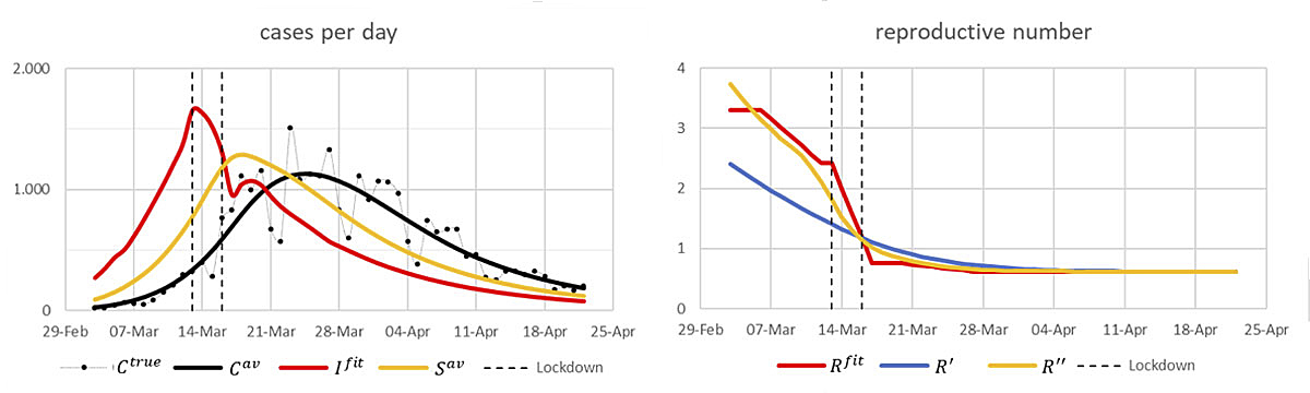
Figure 4 Left: “True” infection numbers (red) and their corresponding expected numbers of cases with symptom onset per day (yellow) and of confirmed cases per day (black). Right: The corresponding ’true’ reproductive numbers (red) and their reconstructions according to the schemes [8] (yellow) and [3] (blue).
We stress that the knowledge of the dates of symptom onset is an advantage, as adopting the same scheme but with dates of confirmation instead of symptom onset, would introduce the ”noise” xa + ya – mʹ, where mʹ is the average time between infection and confirmation, into the true data, and this is clearly more ”noise” than in the scheme based on dates of symptom onset.
In this article we have re-examined a type of scheme used to estimate the effective reproductive numbers R t for COVID-19 with examples of two versions currently in use [3, 8]. These schemes are based on reconstruction of not directly observable data by sampling time lags of observed data from suitable distributions. Noise effects inherent in these schemes smooth the number statistics of the true data. The analysis of thus smoothed number statistics yields stable results and is easier to handle than classical inference methods as applied in [6, 7]. However, under certain circumstances like the current COVID-19 pandemic, the introduced noise effects dominate the information contained in the true data and lead to erroneous interpretations. The simpler approach adopted by [8] performs better than the one used in [3]. Moreover, we point out that adequate knowledge of the date of symptom onset is an advantage.
The appendices are available as a separate file for downloading at https://smw.ch/article/doi/smw.2020.20307.
We thank Nicola Kistler for asking the right question and Erik Böttger, Jürg Fröhlich and Emanuel Wyler for helpful discussions.
The authors have no financial support nor any other potential conflict of interest relevant to this article.
1ETH Zürich. Monitoring COVID-19 spread in Switzerland. [Internet] Available at: https://bsse.ethz.ch/cevo/research/sars-cov-2/real-time-monitoring-in-switzerland.html. Cited on: 2020 May 13
2Swiss National COVID-19 Science Task force. Effective reproductive number. [Internet] Available at: https://ncs-tf.ch/en/situation-report
3 Scire J , Nadeau S , Vaughan T , Brupbacher G , Fuchs S , Sommer J , et al. Reproductive number of the COVID-19 epidemic in Switzerland with a focus on the Cantons of Basel-Stadt and Basel-Landschaft. Swiss Med Wkly. 2020;150:w20271. doi:.https://doi.org/10.4414/smw.2020.20271
4 Abbott S , Hellewell J , Thompson RN , Sherratt K , Gibbs HP , Bosse NI , et al. Estimating the time-varying reproduction number of SARS-CoV-2 using national and subnational case counts. Wellcome Open Res. 2020;5:112. doi:https://doi.org/10.12688/wellcomeopenres.16006.1
5 https://github.com/daenuprobst/covid19-cases-switzerland
6 Lemaitre JC , Perez-Saez J , Azman AS , Rinaldo A , Fellay J . Assessing the impact of non-pharmaceutical interventions on SARS-CoV-2 transmission in Switzerland. Swiss Med Wkly. 2020;150:w20295. doi:.https://doi.org/10.4414/smw.2020.20295
7 Flaxman S , Mishra S , Gandy A , Unwin HJT , Mellan TA , Coupland H , et al.; Imperial College COVID-19 Response Team. Estimating the effects of non-pharmaceutical interventions on COVID-19 in Europe. Nature. 2020. doi:.https://doi.org/10.1038/s41586-020-2405-7
8 an der Heiden M , Hamouda O . Schätzung der aktuellen Entwicklung der SARS-CoV-2-Epidemie in Deutschland - Nowcasting. Epid Bull. 2020;17:10–5. doi:. See https://edoc.rki.de/handle/176904/6650.4 for updated versionhttps://doi.org/10.25646/6692.2
9 Nishiura H , Linton NM , Akhmetzhanov AR . Serial interval of novel coronavirus (COVID-19) infections. Int J Infect Dis. 2020;93:284–6. doi:.https://doi.org/10.1016/j.ijid.2020.02.060
The authors have no financial support nor any other potential conflict of interest relevant to this article.