Potentials and pitfalls of clinical peptidomics and metabolomics

DOI: https://doi.org/10.4414/smw.2013.13801

Introduction

In the past decade, the emerging “-omics” technologies for the rapid profiling of large numbers of peptide and metabolite markers with mass spectrometry evoked great hopes of detecting new disease biomarkers [1]. High-impact publications in the fields of proteomics [2], peptidomics [3] and metabolomics [4] laid the ground for the expectation that it would be possible to broaden the, as yet, very small spectrum of markers available today, especially for the early detection of malignancy, through the use of easy-to-use high-throughput technologies. However, despite major investments in these fields, despite the ever-advancing refinement of the analytical techniques, and despite the broadening and deepening of our pathophysiological knowledge, no new major cancer biomarker has been approved for clinical use in the past 25 years [5, 6]. On the contrary, the above-mentioned ground-breaking publications in particular have been disproved [7–9], after a first closer look at preanalytics, study design and data evaluation. But why did they fail?

To answer this intriguing question, it may be necessary first to illustrate the biomarker concept. The idea behind a diagnostic “biomarker” (amongst other definitions) is to find a measurable entity that sensitively, specifically and without any bias indicates the presence, progression or absence of a disease state or its surrogate [5]. Such entities can be the presence of proteins, peptides or metabolites, as well as changes in their concentrations or ratios thereof, or even complex interactions depicted in similarly complex algorithms. An extensive overview of the different types of biomarkers and the stages of their development was recently published by Ziegler et al. [10]. In proteomics research, markers are usually considered to be proteins produced or shed in lesser or greater amounts by tumour cells than by healthy tissue. In peptidomics, the altered peptides are assumed not only to arise from tumour tissue, but also to be altered in vivo or ex vivo by tumour-specific processes and enzymes such as proteases [11]. In metabolomics, finally, the metabolite markers themselves are not considered as tumour-specific products, but rather their altered correlations and metabolic pathways (e.g. in the context of the well-known Warburg effect [12, 13]) lead to concentrations and patterns of metabolic intermediates or end-products that are different in health and disease [14]. These alterations can be seen as surrogate markers – associated with, but frequently not causally connected to, the underlying disease. In a wider approach, different “-omics” techniques, and even clinical data, can be assembled to create new “meta-markers” from panels of different analytes in order to add predictive value [15, 16], and their complex interactions can be computationally elucidated [17]. The major challenges, however, in the search for such markers, panels, or models thereof, are sensitivity, specificity and the avoidance of bias [18].

Sensitivity

Sensitivity still is a demanding task in proteomics/peptidomics, as well as in metabolomics. In this context, it is the ability of an analytical method to generate “positive” results for a group of individuals defined as “affected”. This can be achieved either when marker concentrations are high enough to be easily detected, or by use of sophisticated technologies capable of tracing even the smallest amount of putative marker analytes slightly above or, in extreme cases, within the noise level [19]. Thus, the two major fields of potential improvement are analytics and evaluation. When the SELDI-TOF methodology (surface-enhanced laser desorption/ionisation mass spectrometry) was clinically introduced 10 years ago, it was – without any doubt – an analytical revolution, but not in terms of sensitivity. Therefore, it was no surprise that the first markers identified from SELDI profiles were highly abundant and very well-known serum proteins or fragments [20]. Regarding the concentration ranges of the conventional tumour markers used hitherto, there might be a factor of 10⁴ gap unbridgeable with contemporary mass spectrometric screening equipment [21]. And even with, for example, conventionally assayed cancer antigen-125 (CA-125), which has a detection limit as low as 1.5 kU/l, for the early detection of ovarian cancer, the “biomarker lead time” might last more than 10 years, as Hori and Gambhir revealed by mathematical modelling of tumour growth, shedding and marker elimination [6, 22].

Although the analytical sensitivity is increased many-fold with any new generation of mass spectrometry instruments, detection limits still remain the major technical challenge in clinical peptidomics and metabolomics [23]. Also, when we started our clinical studies using MALDI-TOF MS (matrix-assisted laser desorption/ionisation mass spectrometry) with pancreatic cancer as a model disease, the only marker we could detect and identify was platelet factor 4 (PF4) [24]. Since PF4 is an analyte clinical chemistry has been acquainted with for many years, we could readily verify our results with a commercially available enzyme-linked immunosorbance assay (ELISA). To enhance selectivity we used in our study one further technique, which has been proposed as a possible way out of the sensitivity dilemma by Hori and Gambhir as well as many others: the generation of compound marker models or “meta-markers” [15, 22, 25, 26]. The idea behind this concept is that different markers can explain different aspects of the overall variance in a dataset by providing different perspectives on a certain disease and, therefore, may exert additive effects when optimally combined together. Besides several limitations recently outlined by Pepe et al. and Pencina [25, 27], and the certain need to keep in mind Occam’s law of parsimony (which states that the exclusion of unnecessary variables probably leads to better models) to avoid data overfitting [28], this definitely is a promising approach to explaining multifactorial phenotypes with multivariate predictors. The measurement of single peptidomic or metabolomic markers may not exceed the selectivity of conventional tumour markers [28]. However, combinations of expression profiling, imaging technologies such as computer tomography, magnetic resonance imaging or positron emission tomography, and even other sources of information about the patient (e.g. epidemiological data), might lead to a substantial increase in sensitivity. In this context, “-omics” technologies, conventional laboratory medicine and imaging should not be seen as separate disciplines, but as complementary approaches to the same diagnostic question. For the merging and modelling of compound “meta-markers”, however, a further abstraction step in medical imaging that resolves image data to qualitative or quantitative features is necessary.

Another approach to increase sensitivity is the use of enrichment techniques in the sampling and sample preparation phase, including in-vivo sampling, optimised extraction methodology and preconcentration steps [29], as well as the application of mass spectrometric ion collection methods such as ion traps [23]. The third way to increase sensitivity might be a radical shift of the researchers’ perspective from molecules shed or modified directly by a tumour or a certain disease towards large-scale meta-effects, which are well known in, for example, malignant disease (sweating, weight loss, etc.), and are mainly metabolism based and, therefore, an optimal target for metabolite profiling and metabolomics [3]. Of course, such metabolic alterations themselves might not be very specific, but there is hope of finding specific patterns based on multiple interactions of diseases with key enzymes of metabolic pathways [30], leading to a set of a few, easy-to-quantitate metabolic markers. Since these metabolic effects are so pronounced that they frequently generate a prima vista phenotype, like malignant cachexia [31], they should be large enough to be detectable with today’s imperfect profiling technology [32].

Specificity

Specificity is the second challenge on the way to the successful implementation of proteomics/peptidomics and metabolomics in clinical diagnostics and practice. Specificity is herein defined as the capability of a marker to assign “negative” values to subjects defined as “nonaffected”. The problem with this definition is that, especially in matched control studies, the “nonaffected” are a highly selected subgroup, of the general population in the case of screening markers and of the patient group in the case of a discriminative disease marker. This may lead to a situation in which a suggested “new” biomarker performs extremely well in a matched-control study environment, but loses all selectivity when used in, for example, a clinical setting with many potential differential diagnoses [27], where the principal differentiation between “healthy” and diseased is trivial. Therefore, when the discriminative power of a proposed biomarker is reported, it is essential to take the composition of the disease and control groups into consideration.

Another problem also depends on the size and composition of the study groups, so-called “overfitting”, which denotes the “overspecification” of a model on the basis of irrelevant variables. If we search, for example, for differences between two groups, we might find “markers” that separate the groups stunningly well, but are not related to the classification criterion itself. Especially when the study groups are small and large numbers of potential “markers” are investigated, the usual 5% error level leads to one statistically “significant” but random marker out of 20, especially when heuristic approaches are applied. For this pitfall, several solution strategies are available. The first is to increase the number of subjects compared: if the number of observed variables is the same, the probability that the differences therein are random decreases. That might sound simple, but to obtain high-quality samples from well-documented patients in a reasonable timeframe can be a real challenge, especially for smaller diagnostic centres. If several variables are under investigation, the corresponding p-values should be adjusted accordingly. Additionally, the study groups should resemble the heterogeneity of the populations for which a “marker” is designed in an optimal way, in order to avoid findings that are selective only for a small subpopulation. The next possibility is the application of split-half [18] or crossover study designs [24], internal cross-validation, or bootstrapping [33]. Although these methods are generally recommended, they nevertheless may be prone to bias [34]. The third and probably best way to avoid overfitting remains totally independent, external validation of the results. That means that the validating group investigates a previously published “marker” with an independent team, independent patients and an independent analytical platform [5, 18]. However, not even this “gold standard” of validation is free of bias, when, for example, the independence is compromised, or only the best datasets or models are reported [34]. In an optimal case, all three solutions should be applied complementarily.

A further, frequently neglected point is that the specificity of a predictive model strongly depends on the selected cut-off, and that even predictive models that perform well lead to wrong decisions if the cut-off level is not set adequately [35]. In a recent publication, Pepe et al. [27] outline another threat to specificity: the distortion of the distribution of relevant risk factors by matching, which can lead to false estimation of the predictive performance of a biomarker when it is correlated to a matched risk factor. Also, the computation of the gain in specificity achieved by incorporating a new marker into an existing model (“added value”) is a nontrivial task far beyond simply detecting a significant difference between receiver operator characteristic (ROC) curves [15, 35, 36].

Avoidance of bias

The third, and probably greatest, challenge in biomarker research is the avoidance of bias. Bias is defined as an unintentional, unconscious, systematic, erroneous association of some characteristic(s) within a group, in a way that distorts comparison with another group [18]. In other words, a covariate we are not aware of. This unawareness is the principal problem of any kind of bias – if we a priori knew (and appropriately remembered) the potential sources of bias, we could address them in the design of our studies. And they are legion! Some of them were already mentioned in the preceding paragraphs, but their range covers the complete process from study concept, subject selection, the preanalytical phase, measurement, postprocessing and interpretation. Especially in metabolomics, which is defined as the unbiased analysis of all metabolites in a defined system [23, 37] and usually performed within observational study designs, the avoidance of bias is critical [38].

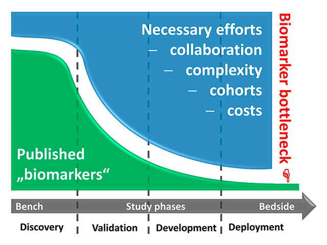
Figure 1

The biomarker bottleneck. During the successive phases of the transition of a biomarker from bench to bedside (roughly segmented into exploratory “discovery”, multicentred “validation”, clinical assay “development”, and large-scale “deployment” phases), the hurdles for successful evolution are steeply increasing. Researchers face exploding costs and complex regulatory requirements, and they have to cooperate with competing groups to gain large and independent validation cohorts. Finally, few – if any – markers can be clinically established.

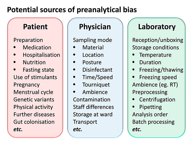
Figure 2

Potential sources of preanalytical bias.

RT = room temperature.

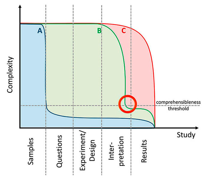
Figure 3

Complexity of the conventional “hypothesis-driven” approach (A) compared with “hypothesis-free” study approaches (B & C). Most of the published metabolomics studies resemble study type C: differences are determined and principal component analysis (PCA) score plots are frequently drawn. But since complexity is not really reduced, interpreting the data and answering the study questions is difficult and sometimes impossible. Study type B includes a complexity reduction step (e.g. variable/model selection, see orange circle) and thereby facilitates interpretation. Elaborate statistics are necessary to perform this reduction, but they are unavoidable since the complexity of the information contained in the “-omics” data usually exceeds human comprehension (the “comprehensibleness threshold” signifies this limit).

Study concept

The fundamental problem in observational studies is “equality at baseline”: the claim that controls and patients in, for example, a metabolomics study are equal in all measurable variables except for disease [18, 38], thus rendering the disease-specific differences obvious. Whereas such equality can be guaranteed by the law of large numbers in an experimental study design when, for example, diseased patients are randomly assigned to one of several treatment strategies, it is nearly impossible to select patients and controls who are perfectly matched in all variables of relevance, especially when the relevance first becomes apparent during the study course. Indeed, by optimally matching patients and controls, researchers create a synthetic “nonclinical” or “nonepidemiological” situation, which impedes evaluation of marker performance by distorting true prevalences and thereby a priori probabilities [27].

Another key question for study design is: to split or not to split? Today, splitting the study cohort into a “training” group in which, for example, discriminatory models are generated, and a “validation cohort”, which is used to verify the diagnostic performance of the marker models, is generally accepted. In principle, there are three ways to perform splitting. First, so-called internal cross-validation, in which a part of the cohort (e.g. 20%) is left out, and the other part (80%) is analysed. The analysis procedure is then repeated four times, each with another 20% left out. The most extreme case of this k-fold cross-validation excludes just one subject at a time and is called the “jack-knife” method. These methods are, however, prone to bias and their inappropriate application might lead to inflated estimates of classification accuracy [34]. The aforementioned split-half approach omits the k-fold resampling and simply uses one part (usually 50%) of the cohort as a training set and the other part as a validation set. But this method also has a severe drawback. Knottnerus and Muris stated that “it only evaluates the degree of random error at the cost of even increasing such error by reducing the available sample size by 50%” [39]. They propose a third way to split cohorts: the “totally independent” and truly external evaluation. In this, the metastudy cohorts consist of independently collected and analysed subcohorts from different centres and investigators. This third way is probably the optimal procedure to detect (and thereafter avoid) sources of bias related to centre-specific features such as different patient preparation, different preanalytical protocols (or their different observance), different analytical methods and different interpretation of the measurement results in the various study centres when they depend on individual ratings. On the other hand, “externality” might be the most difficult task, because many variables have to be fitted across different centres, and researchers have to collaborate with potentially competing groups and rely on the protocol adherence of their colleagues to get the results validated. Another problem might be the opinion of many expert reviewers that it would be necessary to demand “external” validation for any kind of biomarker study, while being unaware that truly “external” means that their claims should be addressed to other, “external” groups.

Another important aspect that Rifai et al. [40] and Ziegler et al. [10] mention is the “staging” of biomarker studies. As in tumour development, the “early stage” studies are small and single-centre, whereas the “late stage” studies include multiple centres and grow to population scale. In the “discovery phase” a first pilot investigation of several tens to a hundred samples are analysed and, usually by means of differential analysis, potential “biomarkers” are identified. Such studies are easy to perform, are (so far) published fast and, once the analytical equipment is available, also not very expensive. The vast majority of published “-omics” biomarker studies can be assigned to this category, although they frequently are not appropriately labelled as “pilot” or “preliminary” investigations. Hence, a huge number of “potential” biomarkers could be available for further validation – which is never done, because the subsequent validation phases are expensive, need larger sample collections (which are frequently not available) and, in the case of multicentre studies, require cooperation with possibly competing researchers. These phases comprise, for example, external validation, assay refinement, prospective evaluation and, finally, the development, approval and deployment of a (commercial) clinical assay (fig. 1). Unfortunately, the financial and regulatory requirements, as well as the risks of failure, of these later stages exceed the capabilities of most research groups, and as long as funding is granted because there is “a lack of biomarkers” (which is essentially wrong, because there is primarily a lack of validated biomarkers), researchers will continue to flood scientific literature with preliminary, nonreplicable and biased “markers”.

A frequently overlooked pitfall is the loss of generalisability. If the cohorts of healthy controls and patients are selected in accordance with very strict selection criteria, they only represent “special cases”. If a model is built thereon, it might perfectly discriminate these cohorts, but after translation into clinical practice, the usual composition of affected and nonaffected cohorts will vary considerably, and the results will not be replicable. The difficulty with this situation is that it cannot be resolved, even with external validation, when the same eligibility criteria are applied in training and validation studies. Therefore, an extensive display of the “descriptives” is mandatory in publications of biomarker studies to enable physicians to evaluate subsequently whether their patients fit into the respective target cohort and are suitable for the diagnostic procedure. In this context, at least three points are important. Firstly, the standardisation, which is necessary without any doubt, should not narrow the patient spectrum down to a collection of “special cases” when a diagnostic method is proposed for general application. In contrast, although the preanalytical influences should be as controlled as possible, the biological variability in the samples should resemble the future target population and therefore include, for example, typical comorbidities in the patient as well as in the control group. Secondly, an evaluation plan should be set up before the sample collection starts. At the moment, many biomarker studies are “passively” designed, based on pre-existing sample collections, which are compared simply because they are available. Samples should be collected prospectively and focused on a specific target, because only under these conditions can they be collected in a way that takes into account all the aforementioned points [41]. Thirdly, biomarker studies should be recorded in a uniform register providing all the information necessary for external scientists to perform validation studies [42, 43].

Preanalytical phase

The first disappointment after the “proteomics hype” arose mainly from preanalytical issues [1]. Basic principles well known in laboratory medicine had to be reinvented when the quest for new disease biomarkers began in the emerging “-omics” technologies. Probably the most famous archetype of a nonreproducible biomarker study was reported in the ground-breaking publication of Petricoin et al. [2], which proposed “an iterative searching algorithm that identified a proteomic pattern that completely discriminated cancer from noncancer”. Two years later, Baggerly et al. [44] reanalysed the datasets, identified many analytical and bioinformatic shortcomings, and finally could not reproduce the results. Another notable example was the suggestion by Xu et al. that lysophosphatidic acid was a biomarker for ovarian cancer [45]; this even led to a failed commercial validation attempt. A few years later, the selectivity of this biomarker was disproved in a subsequent study [46]; as Eleftherios Diamandis states, the uncontrolled leakage of lysophosphatidic acid from blood cells introduced preanalytical biases in the results [5]. In the field of metabolomics, Sreekumar et al. [4] published a widely noticed study on the discovery of the role of sarcosine in prostate cancer progression. However, the findings of an immediate re-evaluation of the results in well-defined samples by Jentzmik et al. [47, 48] suggested that the findings were more likely to be a result of cohort differences rather than true elevations of sarcosine levels in the urine of prostatic cancer patients.

At the time we started proteomics research little was known about the innumerable influencing factors that can hamper and bias comparisons between different patient groups by means of increasingly sensitive mass spectrometric methodology. Nearly anything we could imagine led to a detectable and frequently “significant” difference, especially when the analytes were not absolutely stable and heuristic bioinformatics were applied. We soon realised that preanalytical standardisation is essential, and focused primarily on establishing protocols for different sample materials [49–51] and platforms [52]. However, studies of preanalytical bias can by design only address confounders that are already known. Other sources of bias might appear during proteomic or metabolomic studies, or may become apparent after the study is conducted, for example during exploratory data analysis. Then it becomes very difficult to correct for that bias ex posteriori. To enable the detection of even unknown bias, it might be reasonable to record all preanalytical variables that could have potential impact on the samples and their comparison, and to perform exploratory analysis in advance of any biomarker modelling efforts.

Fields of potential bias (fig. 2) are the patient preparation (e.g. premedication or hospitalisation), nutrition (e.g. fasting or standard diet), the exact mode of sampling itself (e.g. the punctured vein, upright or sitting position), the sampling time (to standardise circadian effects), the sampling material (e.g. the batch and brand of syringes and tubes), the transport conditions of the samples (e.g. time, temperature, acceleration), the complete sample preprocessing (centrifugation, pipetting, etc.), the freezing and thawing speed, the storage temperature and time, and the occurrence of repeated freezing and thawing cycles.

Special attention should be paid to the selection of the sampled biomaterial. For MALDI-TOF peptide profiling of human blood, serum might be a reasonable choice [11, 51], whereas for the investigation of diseases limited to the brain, cerebrospinal fluid can be necessary [50], because the concentrations of the analytes are too low in the peripheral blood. Urine is an optimal material for small molecules excreted by the kidneys. However, dilution, contamination and decay can be high, and can impede analysis and interpretation [53]. For pancreatic disease, pancreatic juice has been proposed as a promising sample type for pilot studies [54], but the invasiveness of its retrieval prohibits its use for screening. In an even more adverse case, the fluid enriched with a potential biomarker might be secluded from the circulation (e.g. in a cyst or abscess), rendering blood-based detection impossible despite high local concentrations.

Additional factors are the time the individual sample waits for analysis when samples are analysed in batches (e.g. in the sample tray of a mass spectrometer, or even the potentially temperature-dependent position on a noncooled tray), the randomness of the analysis order (to avoid continuous “shift” affecting patient and control samples to a different extent), and also the ambient conditions (e.g. air humidity for the cocrystallisation in MALDI-TOF sample preparation).

A possibility to consider for assessing potential influences is the use of internal or external markers, which are added early in the preanalytical pipeline and could be used to quantify sample degradation or alterations during the preanalytical handling. However, such markers themselves introduce bias, and the benefit and the detrimental effects of their use have to be considered very carefully [55].

Measurement

For proteomics/peptidomics, as well as for metabolomics, a large number of analytical platforms are available and the generalisability of their different results is very limited, even within the results from a single platform [56]. In principle, there are two main approaches, the “nontargeted” and the “targeted”. The “nontargeted” approach is usually applied when no prior knowledge about the markers to be found exists and the method is used to detect the widest possible range of differential analytes. The “targeted” approach is selected when a small number of suspected analytes have to be quantified in order to determine exactly the differences between groups. Both approaches have advantages and problems. The “nontargeted” approach allows the detection of hitherto unknown markers, but is (in general) limited in sensitivity and quantitation capabilities, and generates huge amounts of data, which have to be stored, processed, and interpreted. In contrast, the “targeted” approach delivers superior sensitivity and “simple” quantitative data, which are more easily compared between different platforms, but are limited to the analytes the method is tuned for. For both approaches many vendors produce machinery and applications, and the technical development is extremely rapid, leading to a situation in which potential markers are rarely “externally” confirmed, just because the groups having suitable cohorts might not have the same technical platform.

Just as reporting is extremely important in preanalytics, it is likewise essential for the analytical phase. Besides the exact instrument settings (which are frequently displayed in hardly accessible submenus of the device software), data on inter- and intra-day variation and drift, on the reagents and the processing steps already performed in the instrument (e.g. peak alignment, etc.) should be mentioned. Of course, standards have therefore been developed [57, 58], but their observance is not yet strictly enforced by journal editors. A fact that is often ignored is bias caused by the analytical method itself. Mass-spectrometry, for example, is dependent on ionisation, and this process interferes with the analytes and can even destroy the most fragile ones. Other instrument settings, such as column temperature, can also be problematic for a variety of heat-labile molecules [59]. Although metabolomics is defined as the analysis of all metabolites in a certain biological system, there is no analytical platform covering the whole metabolome [37], rendering metabolomics sensu stricto impossible at the moment. Keeping in mind that any metabolomic experiment must be considered at least as partial, a combination of different techniques and analytical platforms might resolve this dilemma, but also introduce distortions in the global picture of the metabolites owing to different platform-dependent susceptibilities to bias. For general standardisation and comparability, the application of reference materials could be helpful, but also extremely difficult because of the sometimes low stability and wide range of metabolites to be covered. Probably the most reasonable approach would be the use of application-specific reference materials in, for example, “lipidomics” or “glycomics” of human plasma [60], which would necessitate international collaborative efforts. Whenever possible, however, “metabolomic” findings should be validated by a transplatform approach, for example by measuring the analyte identified by mass-spectrometry as differentiating between groups also by means of common and easy available routine methods. If this were standard, many false-positive “metabolite markers” could be sorted out before publication and before other groups waste their time on externally validating them.

Another important fact to realise is that no single measurement is exact, and each result has to be considered in a probability range influenced by random and systematic errors. What is common language in laboratory medicine [61] has to be respelled in “-omics” science. Mass spectrometric instruments especially are extremely sensitive to altered ambient conditions, which severely hampers the reproducibility of the results. The measurement of standardised reference samples, the introduction of replicates and the analysis of all study samples in one batch are just a few recommendations to target this problem. In fact, it is necessary to remember that in certain situations measurement errors can sum up and distort any subsequent analysis attempt. On the other hand, this rediscovery of fundamental concepts of accuracy and precision in the emerging “-omics” technologies also offers a chance for conventional laboratory medicine to redefine handling, accessibility and presentation of result uncertainty.

Finally, another yet unsolved problem is how we treat measurements below the limit of detection (LOD). The fact that the area under a mass-spectrometric curve cannot be integrated does not mean that the concentration equals zero. Setting these value to “null” is artificially “left-censoring” the distribution and might lead to negatively biased ROC estimates [62].

Data processing

The data processing phase of clinical peptidomics or metabolomics studies is another, and probably the most challenging, step in the analytical pipeline. The experience needed therein covers not only analytical and technical knowledge, but also profound skills in mathematics, statistics, epidemiology and even programming. The process of familiarisation with these demanding sciences is usually cumbersome, but absolutely necessary to understand and correctly interpret the data transformations and results. Unfortunately, the emerging “-omics” technologies are developing faster than the relevant curricula. Therefore, researchers have to manage awkward data formats, beta-phase tools, programs that were made for other questions and applications, and visualisations that frequently cover more than two dimensions: It needed, for example, several years and enormous efforts until the first R-based MALDI tool was released and able to process *.fid files [63] or ROC curves with confidence bands could be easily and automatically drawn [64]. To compute correlations of metabolic analyses with several measurements of each study participant, we had to adapt a tool originally developed for genetic analyses [65, 66], and the visualisation of the volume under the ROC surface (VUS) had to be drawn using self-made scripts [67], since this feature is still not available in today’s statistical software. Hence it is always reasonable to be cautious when vendors praise their software as a “one-click-to-result” or “one-button” solution. Due to the enormous variability in analytes, methods, platforms, study designs and questions, there is no “standard” metabolomics study that could be completely approached by using a “standard” program, even if the proprietary software solutions pretend to have such capabilities. However, the number of attempts to standardise more and more aspects of the data processing phase is increasing every year, and indeed there are standardised parts, for example the data formats and reporting [57], the data sharing [68] or the validation [69].

A major obstacle for the implementation of general data treatment guidelines is the huge amount of data generated in, for example, metabolomics experiments, which would have to be standardised in all its aspects, comprising several gigabytes of data for the measurement of a single replicate of, for example, human plasma using ultraperformance liquid chromatography (UPLC) quadrupole time-of-flight mass spectrometry (Q-TOF) analytics. Despite their ongoing evolution, standard office computers are at an immediate limit when spectra information from hundreds or thousands of study participants has to be processed comparatively at the same time. Because of the reduction in sensitivity [19], it might not be an optimal recommendation or “solution” to raise the signal-to-noise ratio (s/n), in order to reduce the size of the dataset, rendering it appropriate for a prioriinsufficient 32-bit hard- and soft-ware. The omission of a signal-to-noise ratio cut-off might boost the sensitivity, but it also demands considerable computing power even for small peptidomics datasets [19].

This hardware gap could be bridged by applying the emerging so-called “cloud” technologies [70] or, for example, (GPU-based) parallel computing [71]. Universities (e.g. the UBELIX cluster of the University of Bern), national academies (e.g. the Leibniz Supercomputing Centre in Munich), and institutes (e.g. the Vital-IT of the Swiss Institute of Bioinformatics) can also provide the necessary resources and enable rapid processing as well as thorough evaluation of even large datasets. The development of web-based services is another step in the direction of centralised computing [72], but confidentiality, intellectual property and reproducibility (e.g. by guaranteed availability of the service, proper maintenance, and versioning) are important points that should be clarified in advance. Meanwhile, the first “R”-packages for integrating different “-omics” approaches have been released [73], and given the ultrarapid development, the ever-increasing number of available packages, and the multi- and grid-processing capabilities of this open-source platform, major advances in the analysis of metabolomics and peptidomics data can be expected within the next few years.

Besides the technical preconditions and documentation, the workflow management also is becoming more and more important. Although the individual settings and parameters may vary from study to study, the workflow or “pipeline” itself might be a reasonable target for standardisation [74–76]. As John Quackenbush stated a decade ago, “reporting data transformations is becoming as important as disclosing laboratory methods. Without an accurate description of either of these, it would be difficult, if not impossible, for the results derived from any study to be replicated” [77].

Interpretation

The last, most neglected and also most intellectual phase in clinical metabolomics and peptidomics is the interpretation of the results. The conceptual approach, procedure and subsequent interpretation strongly depend on the aim of the study – typically to search for “biomarkers” to distinguish between different study cohorts – and can include the detection of differences between groups, the evaluation of their significance, the selectivity of analytes or combinations thereof, the added value in comparison or combination with conventional disease markers, or even the evaluation of the noninferiority or superiority of a new marker or model. The farther we step from the trivial “statistically significant differences” approach, the more complicated and challenging become evaluation and interpretation. The principal problem is the reduction of complexity: the huge amount of data we generate with each peptidomics or metabolomics experiment has to be reduced to clinically “usable” statements or information, in the case of biomarker studies typically expressing the probability of a patient being in one of the disease classes. A second aspect is the reduction of the complexity of the biomarker models. The simpler these models are, the more easily they can be implemented in, for example, standard laboratory information systems, and, according to Occam’s law, simpler models are also more likely to be “true”.

There are different strategies for reducing complexity. First, the study design can be focused to answer one specific question. In this setting we expect a very limited set of results, which are easy to interpret and do not need sophisticated statistical evaluation. Frequently, however, the study design is “hypothesis-free” and the full complexity is maintained until data analysis. In this case, interpretation is extremely difficult, and probably impossible, without elaborate multivariate statistical pipelines (fig. 3). Today, most of the proprietary, usually patched-up, software shipped with analytical instruments is focused on exploratory data analysis, for example principal component analysis (PCA) and other variance-based techniques. This software is commonly used to display different groups, classes, or clusters in the dataset as, for example, score plots. What might seem reasonable ‒ and certainly is ‒ for the detection of bias does not, on the other hand, either reduce the amount of input data or answer the right question. In a standard biomarker study setup, the question is not “how many groups are in my sample?”, because one should a priori and by design know how many groups there are, but rather “how can I restrict and condense the data to a clinically applicable “meta-marker”, which predicts assignment to already known classes?”. In this situation, the common approach of exploratory data analysis might be insufficient alone and should be at least complemented by an inferential strategy. This transition from exploration to inference is a crucial step in the “-omics” evolution. The problem is no longer the sheer amount of data, which can be processed by powerful computing tools. Rather, it is the amount of information that can be derived from these data and which has to be disentangled and reduced to the essential. Unfortunately, there is a “comprehensibleness threshold”. Human perception of complex coherences may be very limited, and for the acceptance of peptidomic or metabolomic data at the patient’s bedside it seems essential to provide information condensed enough to enable a prima vista understanding of a marker model, as well as simple application for the clinician. For these “final” interpretation steps, new statistical concepts and computational options are emerging: For the modelling of clinical outcome on the basis of correlated functional biomarkers, a new Bayesian approach was suggested by Long et al. [78]. For the incorporation of replicate information into correlation estimates, Zhu et al. [66] proposed the R-based CORREP package, which can be applied not only to genetic data, but also to metabolite data [65]. New comparative study designs have stimulated the development of tools for the simultaneous statistical evaluation of diagnostic markers in multiclass settings [79] and the extension of the conventional ROC curve to the third dimension [80].

In addition to the selectivity of any kind of profile or marker its “added value” as compared with the measurement of the standard disease markers is becoming increasingly important as “-omics” diagnostics come closer to the bedside and clinicians have to balance effort and benefit [15, 81]. Noninferiority and equivalence testing also serve as pivotal techniques when the introduction of a new marker or panel is to be considered, and today’s computational capacities enable even computationally intensive confidence interval-based approaches [67, 82] to be calculated.

Another important feature implemented in recent evaluation tools is the display of the uncertainty inherent to any modelling approach. With increasing size of our datasets, the probability that these contain more than one predictive model increases, a fact that still is neglected by many standard evaluation procedures [67, 83, 84]. Also avoiding “false positive” discoveries [85] and, especially in the field of metabolomics, the implementation of pathway data into modelling procedures and the extraction of pathway alterations from the metabolic data [86] will play an ever growing role.

Conclusion

Whether all the massive investments made in peptidomics and metabolomics will condense down to one single clinically useful marker cannot be foreseen at the moment – and considering the smouldering “success” of proteomics it is certainly justifiable to be in doubt – but besides opening a window into the disease specificity of degradation processes and metabolic pathway alterations, clinical peptidomics and metabolomics drive the development of new concepts for the handling of huge “-omics” datasets containing vast amounts of implied biological and pathway information – an academic process quite independent of the analytical improvements introduced by the diagnostics industry. As relatively recent technologies they are still suffering from the many imperfections, insufficiencies and intricacies genomics and proteomics went through before. But it is also a chance – to learn from errors already committed, as well as to apply creatively existing tools and techniques and develop new ones for extended needs. The real challenge is still ahead: to integrate and simultaneously condense results from all the different “-omics” subdisciplines and even conventional analytics to create new, superior “meta-markers”.

References

  1 Master SR. Diagnostic proteomics: back to basics? Clin Chem. 2005;51(8):1333–4.

  2 Petricoin EF, Ardekani AM, Hitt BA, et al. Use of proteomic patterns in serum to identify ovarian cancer. Lancet. 2002;359(9306):572–7.

  3 Ala-Korpela M, Kangas AJ, Soininen P. Quantitative high-throughput metabolomics: a new era in epidemiology and genetics. Genome Med. 2012;4(4):36.

  4 Sreekumar A, Poisson LM, Rajendiran TM, et al. Metabolomic profiles delineate potential role for sarcosine in prostate cancer progression. Nature. 2009;457(7231):910–4.

  5 Diamandis EP. Cancer biomarkers: can we turn recent failures into success? J Natl Cancer Inst. 2010;102(19):1462–7.

  6 Konforte D, Diamandis EP. Is early detection of cancer with circulating biomarkers feasible? Clin Chem. 2013;59(1):35–7.

  7 Diamandis EP. Letter to the Editor about Differential exoprotease activities confer tumor-specific serum peptidome. J Clin Invest. 2006;116(1).

  8 Sorace JM, Zhan M. A data review and re-assessment of ovarian cancer serum proteomic profiling. BMC Bioinformatics. 2003;4:24.

  9 Struys EA, Heijboer AC, van Moorselaar J, et al. Serum sarcosine is not a marker for prostate cancer. Ann Clin Biochem. 2010;47(Pt 3):282.

10 Ziegler A, Koch A, Krockenberger K, et al. Personalized medicine using DNA biomarkers: a review. Hum Genet. 2012;131(10):1627–38.

11 Villanueva J, Shaffer DR, Philip J, et al. Differential exoprotease activities confer tumor-specific serum peptidome patterns. J Clin Invest. 2006;116(1):271–84.

12 Fernie AR, Trethewey RN, Krotzky AJ, et al. Metabolite profiling: from diagnostics to systems biology. Nat Rev Mol Cell Biol. 2004;5(9):763–9.

13 Warburg O. Über den Stoffwechsel der Tumorzelle. J Mol Med. 1925;4(12):534–6. German.

14 Zhang A, Sun H, Wang X. Serum metabolomics as a novel diagnostic approach for disease: a systematic review. Anal Bioanal Chem. 2012;404(4):1239–45.

15 Boulesteix AL, Sauerbrei W. Added predictive value of high-throughput molecular data to clinical data and its validation. Brief Bioinform 2011;12(3):215–29.

16 Zhu CS, Pinsky PF, Cramer DW, et al. A framework for evaluating biomarkers for early detection: validation of biomarker panels for ovarian cancer. Cancer Prev Res. (Phila) 2011;4(3):375–83.

17 Blair RH, Kliebenstein DJ, Churchill GA. What can causal networks tell us about metabolic pathways? PLoS Comput Biol. 2012;8(4):e1002458.

18 Ransohoff DF. Bias as a threat to the validity of cancer molecular-marker research. Nat Rev Cancer. 2005;5(2):142–9.

19 Conrad TOF, Leichtle A, Hagehülsmann A, et al. Beating the Noise: New Statistical Methods for Detecting Signals in MALDI-TOF Spectra Below Noise Level. In: R. Berthold M, Glen R, Fischer I, (eds). Computational Life Sciences II: Springer Berlin Heidelberg; 2006, 119–128.

20 Diamandis EP. Oncopeptidomics: a useful approach for cancer diagnosis? Clin Chem. 2007;53(6):1004–6.

21 Makawita S, Diamandis EP. The bottleneck in the cancer biomarker pipeline and protein quantification through mass spectrometry-based approaches: current strategies for candidate verification. Clin Chem. 2010;56(2):212–22.

22 Hori SS, Gambhir SS. Mathematical model identifies blood biomarker-based early cancer detection strategies and limitations. Sci Transl Med. 2011;3(109):109ra116.

23 Becker S, Kortz L, Helmschrodt C, et al. LC-MS-based metabolomics in the clinical laboratory. J Chromatogr B Analyt Technol Biomed Life Sci. 2012;883–4:68–75.

24 Fiedler GM, Leichtle AB, Kase J, et al. Serum peptidome profiling revealed platelet factor 4 as a potential discriminating Peptide associated with pancreatic cancer. Clin Cancer Res. 2009;15(11):3812–9.

25 Pencina MJ. Caution is needed in the interpretation of added value of biomarkers analyzed in matched case control studies. Clinical Chemistry. 2012;8(58):1176–8.

26 Pencina MJ, D’Agostino RB, Sr., D’Agostino RB, Jr., et al. Evaluating the added predictive ability of a new marker: from area under the ROC curve to reclassification and beyond. Stat Med. 2008;27(2):157–72; discussion 207–12.

27 Pepe MS, Fan J, Seymour CW, et al. Biases introduced by choosing controls to match risk factors of cases in biomarker research. Clin Chem. 2012;58(8):1242–51.

28 Leichtle AB, Nuoffer JM, Ceglarek U, et al. Serum amino acid profiles and their alterations in colorectal cancer. Metabolomics 2012;8(4):643–53.

29 Vuckovic D. Current trends and challenges in sample preparation for global metabolomics using liquid chromatography-mass spectrometry. Anal Bioanal Chem. 2012;403(6):1523–48.

30 Dong X, Tang H, Hess KR, et al. Glucose metabolism gene polymorphisms and clinical outcome in pancreatic cancer. Cancer. 2011;117(3):480–91.

31 Tsoli M, Robertson G. Cancer cachexia: malignant inflammation, tumorkines, and metabolic mayhem. Trends Endocrinol Metab. 2012.

32 Patterson AD, Maurhofer O, Beyoglu D, et al. Aberrant lipid metabolism in hepatocellular carcinoma revealed by plasma metabolomics and lipid profiling. Cancer Res. 2011;71(21):6590–600.

33 Steyerberg EW, Harrell FE, Jr., Borsboom GJ, et al. Internal validation of predictive models: efficiency of some procedures for logistic regression analysis. J Clin Epidemiol. 2001;54(8):774–81.

34 Castaldi PJ, Dahabreh IJ, Ioannidis JP. An empirical assessment of validation practices for molecular classifiers. Brief Bioinform. 2011;12(3):189–202.

35 Steyerberg EW, Pencina MJ, Lingsma HF, et al. Assessing the incremental value of diagnostic and prognostic markers: a review and illustration. Eur J Clin Invest. 2012;42(2):216–28.

36 Demler OV, Pencina MJ, D’Agostino RB, Sr. Misuse of DeLong test to compare AUCs for nested models. Stat Med. 2012;31(23):2577–87.

37 Christians U, Klawitter J, Hornberger A. How unbiased is non-targeted metabolomics and is targeted pathway screening the solution? Curr Pharm Biotechnol. 2011;12(7):1053–66.

38 Ransohoff DF, Gourlay ML. Sources of bias in specimens for research about molecular markers for cancer. J Clin Oncol. 2010;28(4):698–704.

39 Knottnerus JA, Muris JW. Assessment of the accuracy of diagnostic tests: the cross-sectional study. J Clin Epidemiol. 2003;56(11):1118–28.

40 Rifai N, Gillette MA, Carr SA. Protein biomarker discovery and validation: the long and uncertain path to clinical utility. Nat Biotechnol. 2006;24(8):971–83.

41 Thomas L, Peterson ED. The value of statistical analysis plans in observational research: defining high-quality research from the start. JAMA. 2012;308(8):773–4.

42 Andre F, McShane LM, Michiels S, et al. Biomarker studies: a call for a comprehensive biomarker study registry. Nat Rev Clin Oncol. 2011;8(3):171–6.

43 Ioannidis JP. The importance of potential studies that have not existed and registration of observational data sets. JAMA. 2012;308(6):575–6.

44 Baggerly KA, Morris JS, Coombes KR. Reproducibility of SELDI-TOF protein patterns in serum: comparing datasets from different experiments. Bioinformatics. 2004;20(5):777–85.

45 Xu Y, Shen Z, Wiper DW, et al. Lysophosphatidic acid as a potential biomarker for ovarian and other gynecologic cancers. JAMA. 1998;280(8):719–23.

46 Baker DL, Morrison P, Miller B, et al. Plasma lysophosphatidic acid concentration and ovarian cancer. JAMA. 2002;287(23):3081–2.

47 Jentzmik F, Stephan C, Lein M, et al. Sarcosine in prostate cancer tissue is not a differential metabolite for prostate cancer aggressiveness and biochemical progression. J Urol. 2011;185(2):706–11.

48 Jentzmik F, Stephan C, Miller K, et al. Sarcosine in urine after digital rectal examination fails as a marker in prostate cancer detection and identification of aggressive tumours. Eur Urol. 2010;58(1):12–8; discussion 20–1.

49 Baumann S, Ceglarek U, Fiedler GM, et al. Standardized approach to proteome profiling of human serum based on magnetic bead separation and matrix-assisted laser desorption/ionization time-of-flight mass spectrometry. Clin Chem. 2005;51(6):973–80.

50 Bruegel M, Planert M, Baumann S, et al. Standardized peptidome profiling of human cerebrospinal fluid by magnetic bead separation and matrix-assisted laser desorption/ionization time-of-flight mass spectrometry. J Proteomics. 2009;72(4):608–15.

51 Fiedler GM, Baumann S, Leichtle A, et al. Standardized peptidome profiling of human urine by magnetic bead separation and matrix-assisted laser desorption/ionization time-of-flight mass spectrometry. Clin Chem. 2007;53(3):421–8.

52 Brauer R, Leichtle A, Fiedler G, et al. Preanalytical standardization of amino acid and acylcarnitine metabolite profiling in human blood using tandem mass spectrometry. Metabolomics. 2011;7(3):344–52.

53 Fiedler GM, Ceglarek U, Leichtle A, et al. Standardized preprocessing of urine for proteome analysis. Methods Mol Biol. 2010;641:47–63.

54 Zhou L, Lu Z, Yang A, et al. Comparative proteomic analysis of human pancreatic juice: methodological study. Proteomics. 2007;7(8):1345–55.

55 Findeisen P, Costina V, Yepes D, et al. Functional protease profiling with reporter peptides in serum specimens of colorectal cancer patients: demonstration of its routine diagnostic applicability. J Exp Clin Cancer Res. 2012;31:56.

56 Pelikan R, Bigbee WL, Malehorn D, et al. Intersession reproducibility of mass spectrometry profiles and its effect on accuracy of multivariate classification models. Bioinformatics. 2007;23(22):3065–72.

57 Goodacre R, Broadhurst D, Smilde A, et al. Proposed minimum reporting standards for data analysis in metabolomics. Metabolomics. 2007;3(3):231–41.

58 Taylor CF, Paton NW, Lilley KS, et al. The minimum information about a proteomics experiment (MIAPE). Nat Biotechnol. 2007;25(8):887–93.

59 Ekblad L, Baldetorp B, Ferno M, et al. In-source decay causes artifacts in SELDI-TOF MS spectra. J Proteome Res. 2007;6(4):1609–14.

60 Beasley-Green A, Bunk D, Rudnick P, et al. A proteomics performance standard to support measurement quality in proteomics. Proteomics. 2012;12(7):923–31.

61 Petersen PH, Stockl D, Westgard JO, et al. Models for combining random and systematic errors. assumptions and consequences for different models. Clinical chemistry and laboratory medicine : CCLM / FESCC. 2001;39(7):589–95.

62 Perkins NJ, Schisterman EF, Vexler A. Generalized ROC curve inference for a biomarker subject to a limit of detection and measurement error. Stat Med. 2009;28(13):1841–60.

63 Gibb S, Strimmer K. MALDIquant: a versatile R package for the analysis of mass spectrometry data. Bioinformatics. 2012;28(17):2270–1.

64 Robin X, Turck N, Hainard A, et al. pROC: an open-source package for R and S+ to analyze and compare ROC curves. BMC Bioinformatics. 2011;12:77.

65 Leichtle AB, Helmschrodt C, Ceglarek U, et al. Effects of a 2-y dietary weight-loss intervention on cholesterol metabolism in moderately obese men. Am J Clin Nutr. 2011;94(5):1189–95.

66 Zhu D, Li Y, Li H. Multivariate correlation estimator for inferring functional relationships from replicated genome-wide data. Bioinformatics. 2007;23(17):2298–305.

67 Leichtle A, Ceglarek U, Weinert P, et al. Pancreatic carcinoma, pancreatitis, and healthy controls: metabolite models in a three-class diagnostic dilemma. Metabolomics. 2013;9:677–87.

68 Field D, Sansone SA, Collis A, et al. Megascience. Omics data sharing. Science 2009;326(5950):234–6.

69 Ioannidis JP, Khoury MJ. Improving validation practices in “omics” research. Science. 2011;334(6060):1230–2.

70 Mohammed Y, Mostovenko E, Henneman AA, et al. Cloud parallel processing of tandem mass spectrometry based proteomics data. J Proteome Res. 2012;11(10):5101–8.

71 Conrad T. New statistical algorithms for the analysis of mass spectrometry time-of-flight mass data with applications in clinical diagnostics. Free University of Berlin Institute of Mathematics 2008.

72 Xia J, Mandal R, Sinelnikov IV, et al. MetaboAnalyst 2.0 – a comprehensive server for metabolomic data analysis. Nucleic Acids Res. 2012;40(Web Server issue):W127–33.

73 Le Cao KA, Gonzalez I, Dejean S. integrOmics: an R package to unravel relationships between two omics datasets. Bioinformatics. 2009;25(21):2855–6.

74 de Bruin JS, Deelder AM, Palmblad M. Scientific workflow management in proteomics. Mol Cell Proteomics. 2012;11(7):M111 010595.

75 Junker J, Bielow C, Bertsch A, et al. TOPPAS: a graphical workflow editor for the analysis of high-throughput proteomics data. J Proteome Res 2012;11(7):3914-20.

76 Sung J, Wang Y, Chandrasekaran S, et al. Molecular signatures from omics data: from chaos to consensus. Biotechnol J. 2012;7(8):946–57.

77 Quackenbush J. Microarray data normalization and transformation. Nat Genet. 2002;32(Suppl):496–501.

78 Long Q, Zhang X, Zhao Y, et al. Modeling clinical outcome using multiple correlated functional biomarkers: A Bayesian approach. Stat Methods Med Res. 2012.

79 Luo J, Xiong C. DiagTest3Grp: An R Package for Analyzing Diagnostic Tests with Three Ordinal Groups. Journal of Statistical Software. 2012;51(3).

80 Nakas CT, Alonzo TA, Yiannoutsos CT. Accuracy and cut-off point selection in three-class classification problems using a generalization of the Youden index. Stat Med. 2010;29(28):2946–55.

81 Moons KG, de Groot JA, Linnet K, et al. Quantifying the added value of a diagnostic test or marker. Clin Chem. 2012;58(10):1408–17.

82 Tunes da Silva G, Logan BR, Klein JP. Methods for equivalence and noninferiority testing. Biol Blood Marrow Transplant. 2009;15(1 Suppl):120–7.

83 Jesneck JL, Mukherjee S, Yurkovetsky Z, et al. Do serum biomarkers really measure breast cancer? BMC Cancer. 2009;9:164.

84 Yeung KY, Bumgarner RE, Raftery AE. Bayesian model averaging: development of an improved multi-class, gene selection and classification tool for microarray data. Bioinformatics. 2005;21(10):2394–402.

85 Broadhurst D, Kell D. Statistical strategies for avoiding false discoveries in metabolomics and related experiments. Metabolomics. 2006;2(4):171–96.

86 Krumsiek J, Suhre K, Illig T, et al. Bayesian independent component analysis recovers pathway signatures from blood metabolomics data. J Proteome Res. 2012;11(8):4120–31.